Ecosystem Modeling
Ecosystem Modeling with Atlantis
Lansing Perng, Mariska Weijerman, Kirsten Leong, Lucia Hošeková, and Kirsten L.L. Oleson
![[Alt Text]](assets/img/lansing/project_workflow.png)
We assessed how climate change may affect ecosystem goods and services in the Main Hawaiian Islands using the Atlantis ecosystem model. To build the model environment we applied high-resolution climate projections under three scenarios: optimistic, intermediate and pessimistic. We also calibrated a fishing submodel with historical catch data. With these inputs the Atlantis model projects realistic ecosystem and fishery outcomes.
Model dynamics in Atlantis are shaped by food web interactions. The pyramid shows a simplified version of the 59 functional groups included in the model. Most groups are organized by feeding and habitat type. Some key fish, coral and megafauna species are represented in more detail to capture their ecological importance.
![[Alt Text]](assets/img/lansing/atlantis_trophic_pyramid.png)
![[Alt Text]](assets/img/lansing/coral_bleaching.png)
For model parameterization we set the initial coral bleaching threshold at 28 °C, which is standard for Hawaiʻi. The model includes an assumed temperature adaptation of 0.2 °C per decade. We also applied species-specific pH responses developed by a previous Atlantis team through a meta-analysis of sensitivity studies in the tropical Pacific.
Atlantis is a box model built from user-defined polygons. In our region the polygons follow fishing zones and habitat. The model includes 93 boxes. Of these, 79 are dynamic boxes where ecological and biological changes occur and data are recorded. The remaining 14 are non-dynamic boxes representing islands and pelagic areas that provide inputs to the dynamic boxes. Each box has four depth layers based on light. The photic zone extends to 30 m, the mesophotic to 150 m, and the subphotic to 400 m, with a sediment layer below.
![[Alt Text]](assets/img/lansing/atlantis_boxes_map.png)
![[Alt Text]](assets/img/lansing/corals_biomass.png)
Coral biomass declines under all climate scenarios, with sharper losses in higher emission pathways. Only the low-emission scenario (SSP1) stays above 50% of the initial biomass by 2100. In the high-emission scenario (SSP3), biomass falls to about 25% of the starting level. The coral response is more immediate to rising temperature, with consistent declines beginning early in the simulation. The effect of acidification is slower, becoming more pronounced after 2050 as pH trajectories diverge. This pattern reflects observed climate stressors, where high temperatures trigger rapid mortality through bleaching, while acidification gradually reduces calcification rates.
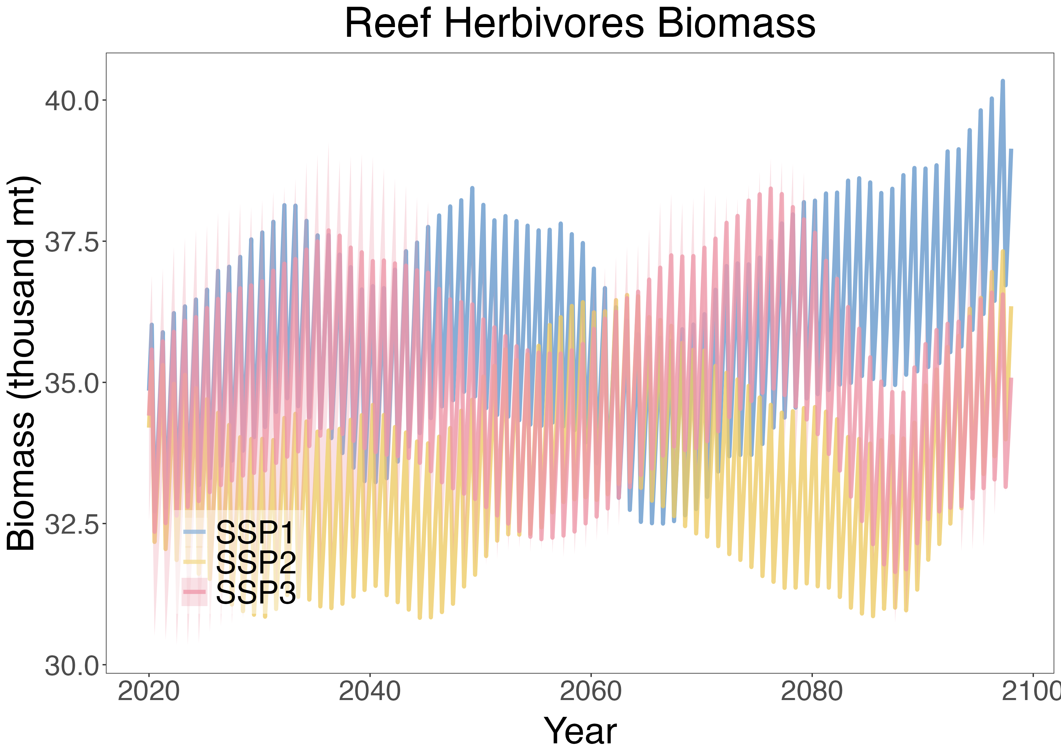
Reef herbivore biomass remained relatively stable across all climate scenarios and increased under SSP1, the low-emission pathway. This outcome reflects the balance between food availability and habitat complexity. In SSP1, herbivores had fewer food resources from macroalgae and turf, yet biomass increased. This likely results from reduced coral loss, which preserved habitat structure and supported herbivore populations.
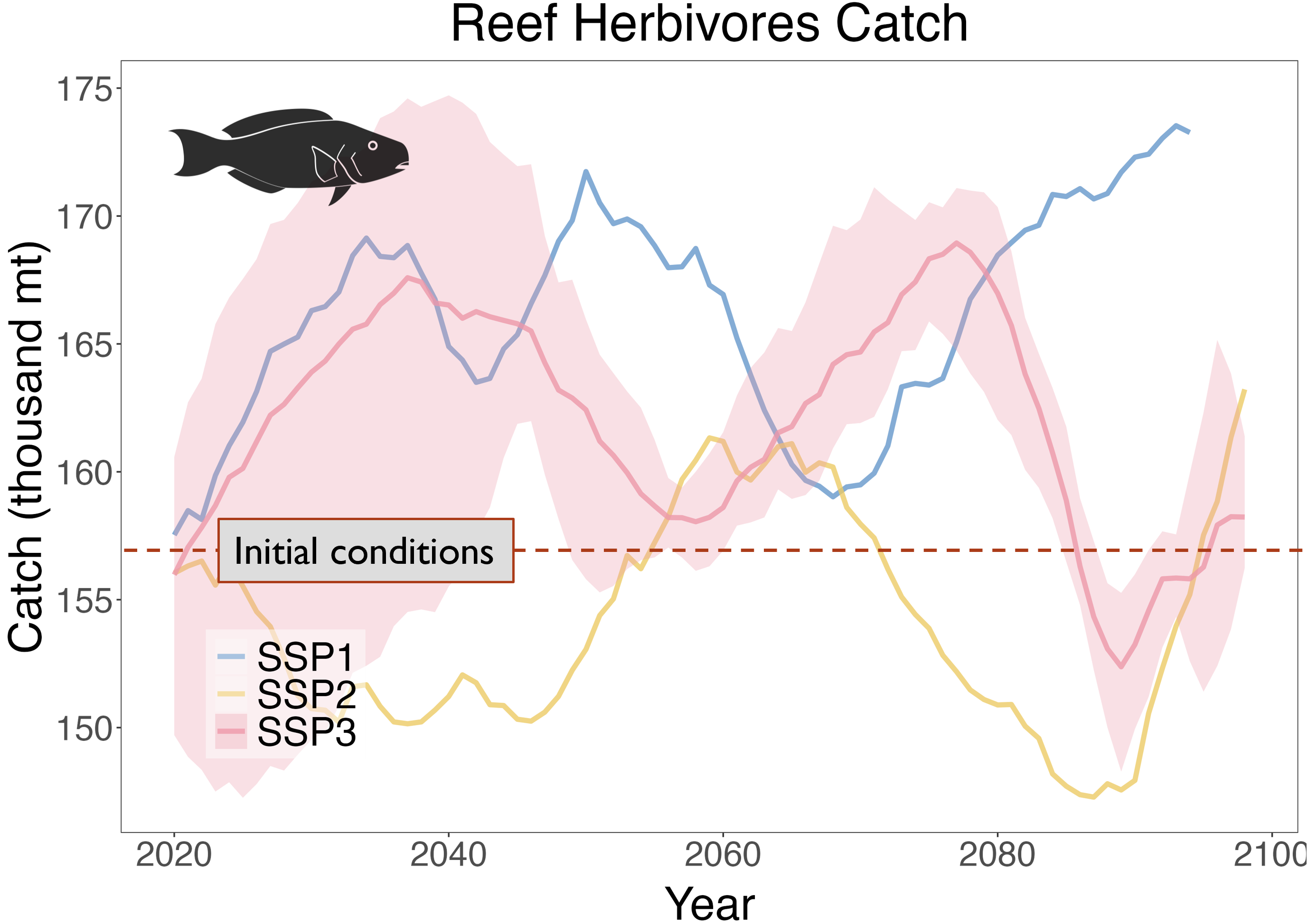
Catch of reef herbivores shows clearer differences across scenarios toward the end of the century. Under SSP2 and SSP3, catches remain close to initial levels with fluctuations over time. In contrast, SSP1 shows an increase above initial catch, reflecting the higher herbivore biomass maintained in the low-emission scenario.
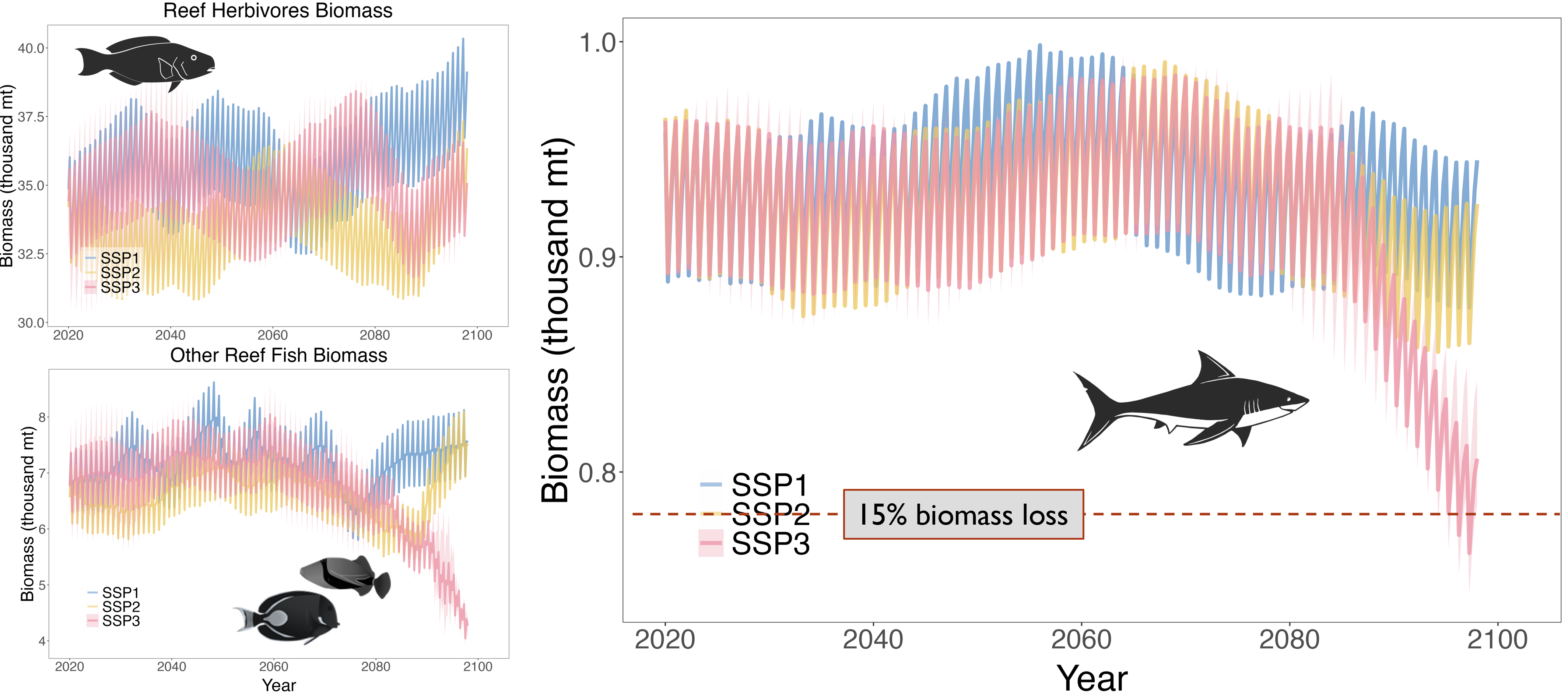
Apex predators in the model include sharks, monk seals and dolphins. Their biomass remains relatively stable across scenarios until late in the century. Under SSP3, the high-emission pathway, biomass declines by about 15%. This decline likely reflects coral loss and the associated reduction in reef fish populations, which lowers prey availability for top predators.
Spatial patterns under SSP3, the high-emission scenario, show strong declines in coral cover through time. The animation on the left tracks coral cover, while herbivore density is shown on the right. In the top panels, pH (left) and temperature (right) highlight the environmental drivers behind these changes. Coral cover remains relatively stable early in the century but drops to very low levels in the second half as warming and acidification intensify.
Coral decline is closely linked with spatial patterns of pH and temperature. The most severe declines occur on the southwest sides of the islands, where waters are warmer and more acidic. These areas show the strongest overlap between climate stressors and coral loss.
Herbivore distributions also shift under SSP3. Over time, biomass concentrates along the northeast shores of the islands, where waters are cooler and coral cover persists. These areas provide more stable habitat and food resources as other regions decline.
The model results show substantial coral declines, with biomass loss increasing under more intense climate scenarios. Differences among pathways were clear, with herbivores reaching their highest levels in SSP1 and apex predators dropping lowest in SSP3. Spatial patterns of biological change mirrored climate trends across the islands, with the strongest impacts where waters warmed most and pH declined. Overall, ecosystem declines intensified with climate stress, beginning at the base of the food web and cascading upward from corals and algae to top predators.